Jupyter notebooks
After this chapter, the students can write and execute Jupyter notebooks. On those notebooks, they can utilise the Markdown syntax to create basic formatting.

Notebooks in science
In any wet-lab, it is essential to keep notes of the experiments and results. That hasn’t always been so in computational analyses but the thinking has radically changed and new tools have been developed for the documentation of computational analysis steps. Probably the most widely used of these tools is Jupyter and its notebooks.
A Jupyter notebook consists of cells that may contain text in Markdown format or programming code understood by the chosen kernel. The original kernel was Python but nowadays kernels for many other programming languages are available, including R. There are command-line tools to convert the notebooks into various formats but we won’t discuss them here; many of the functionalities are available in the web interface. However, as the notebook can be converted to other formats and then processed with tools designed for them (e.g. to LaTeX and then compiled to pdf), the Jupyter notebooks also contain an option to write ‘raw’ code directly for these downstream tools. Here, we focus on ‘Markdown’ and ‘Code’ cells only.
A Jupyter notebook for temperature data analysis
Let’s assume that, in a project utilising temperature data, somebody gets fed up with downloading data manually through a web interface and proposes that another data source with an easy-to-use REST API is used instead. It’s decided that before making the decision to switch to the new data source, it’s good to compare the data obtained from the two places. The person doing the task decides to write her work as a Jupyter notebook; once finished, she will share this notebook – containing both the results and the means for obtaining them in one package – with her colleagues. If they so wish, the colleagues can independently replicate the results using the Jupyter notebook only.
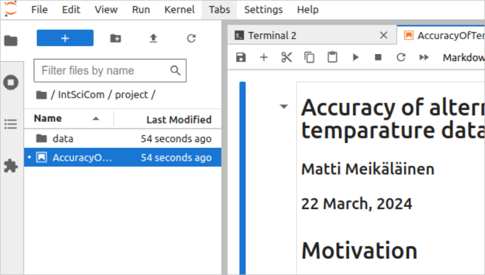
The resulting notebook can be be found in ~/IntSciCom/project/AccuracyOfTemperatureData.ipynb and opened using the file browser in the Jupyter interface
Clicking the first cell selects it (indicated by the blue bar on the left) and the pull-down menu for the “Cell type” in the top shows that the cell is treated as Markdown-formatted text. By double-clicking the cell, one can reveal the underlying Markdown code:
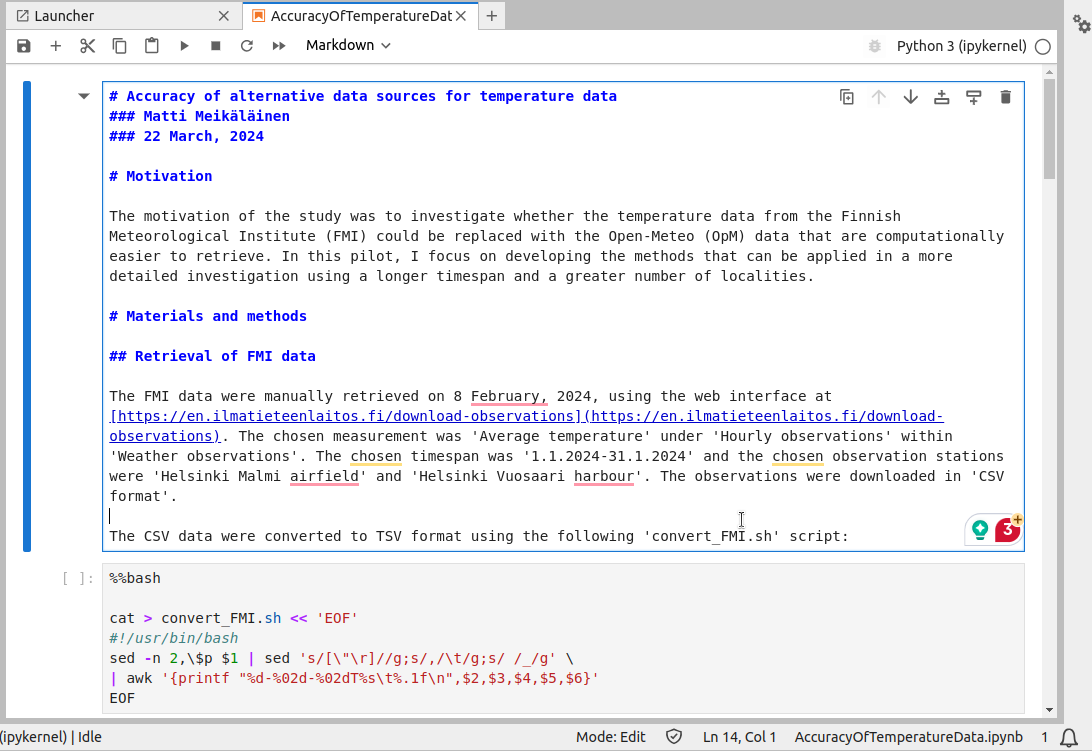
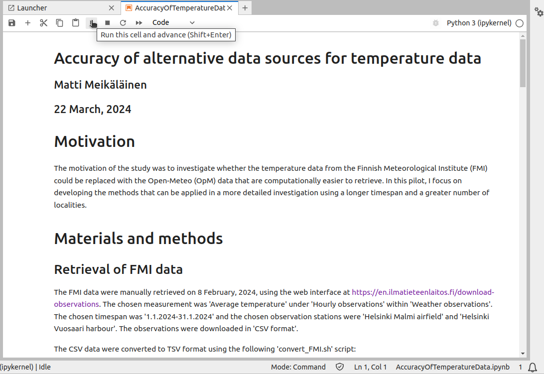
Markdown is meant to be human-readable in the raw format. Here, the headings of different level are indicated by hash characters (#), one hash meaning the first level heading, two hashes the second level etc. Hyperlinks are created with [text](URL), i.e. having the visible text first in square brackets and the URL then in normal brackets. (Above, the URL is repeated.) The cell can be executed by pressing Ctrl+Enter, clicking the triangle in the top bar or selecting “Run” -> “Run selected cell” from the top menu. That now converts the Markdown to a more fancy look:
The next cell is of the type “Code”. The notebook uses the Python 3 kernel (indicated at the bottom of the window) to run the code but this piece of code is clearly written in bash. Indeed, the cell starts with the text “%%bash” which tells Jupyter to run it on the command line as bash code. The code looks familiar from the earlier exercises:
cat > convert_FMI.sh << 'EOF'
#!/usr/bin/bash
sed -n 2,\$p $1 | sed 's/[\"\r]//g;s/,/\t/g;s/ /_/g' \
| awk '{printf "%d-%02d-%02dT%s\t%.1f\n",$2,$3,$4,$5,$6}'
EOF
It writes the pipeline consisting of sed and awk commands to a script file called convert_FMI.sh. In the next code cell, this script is used to convert the manually downloaded FMI data to the OpM format. Similarly to Markdown cells, the Code cells can be executed by pressing Ctrl+Enter, clicking the triangle in the top bar or selecting “Run” -> “Run selected cell” from the top menu.
One could run the Code cells manually one at a time, or one can all of them in order by selecting “Run” -> “Run All Cells” from the top menu. If you do that, you replicate the analysis exactly as someone had done before. This is not the only way to do the investigation and these are not fine-tuned and optimised commands for doing the different steps. (One reason is that I personally don’t know Python very well.) Nevertheless, this is reproducible research at its best.
Sharing Jupyter notebooks
The notebook can be downloaded by right-clicking the notebook file in the file browser and selecting “Download”, or through “File” -> “Download” in the top menu. However, these analyses rely on data that were manually downloaded and, to fully replicate the analyses, they also have to be shared. For maximal compatibility, we can pack them using zip:
> cd ~/IntSciCom/project/
> zip Project.zip AccuracyOfTemperatureData.ipynb data/*csv
Now, the zip-file can be downloaded through the file browser:
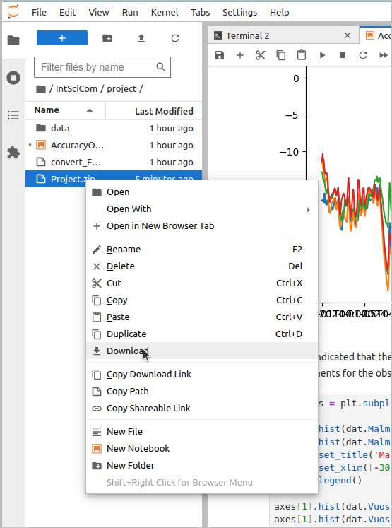
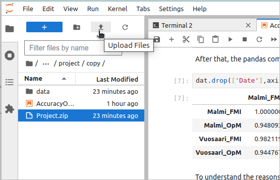
When this zip-file is unpacked, the relative positions of the notebook file and the data files are preserved and the analysis steps can be replicated by running all the cells of the notebook. Note that the file also allows uploading files to the server; this done by clicking the up-arrow symbol in the file browser’s top bar:
An alternative for a fully reproducible notebook is to share the analyses as a pdf-formatted report. This can be done by selecting “File” -> “Save and Export Notebook As” -> “PDF”. However, this adds a title and date in the beginning of the document and doesn’t provide any possibility to edit the properties of the resulting pdf-document. My preferred way is to export the notebook as “HTML” (through “File” -> “Save and Export Notebook As” -> “HTML”) and then opening this html-file in a web browser. This can then be printed through the web browser and e.g. the page margins can be adjusted. The resulting report may then look like this.
Learning the basics of Jupyter & Markdown
The point of Jupyter notebooks is to mix Markdown-formatted text and code. The default language for the code is Python but often the Jupyter installation provides “kernels” for many languages. I personally prefer Jupyter when working with R analyses.
The Markdown format is easy and useful also outside the Jupyter. As an example of that, this course material is written in Markdown and then converted to a web page using quarto. I traditionally have written my papers in LaTeX (often using Overleaf) but have also tested writing them in Markdown and then compiling to pdf with quarto. For the writing, I use Visual Studio Code with plugins for quarto and spelling/grammar checking. It may sound a weird combination for writing texts but it works very well!
The Markdown format is explained at https://www.markdownguide.org/basic-syntax/. A gentle introduction to Jupyter can be found e.g. at https://www.dataquest.io/blog/jupyter-notebook-tutorial/. Inspired by an example there, you could go to the bottom of the existing Jupyter notebook and hover the mouse pointer until you see the text “Click to add a cell”. Do as advised, copy-paste the text below in the cell and press Ctrl+Enter (or Shift+Enter, or click the triangle icon or select “Run” -> “Run Selected Cell”).
# This is a level 1 heading
## This is a level 2 heading
This is some plain text that forms a paragraph. Add emphasis via **bold** or *italic*.
Paragraphs must be separated by an empty line.
* Sometimes we want to include lists.
* Which can be bulleted using asterisks.
1. Lists can also be numbered.
2. If we want an ordered list.
[It is possible to include hyperlinks](https://www.example.com)
Inline code uses single backticks: `foo()`, and code blocks use triple backticks:
```
bar()
```
Or can be indented by 4 spaces:
foo()
And finally, adding images is easy: 
For the Python programming language, the University of Helsinki provides a MOOC at https://programming-24.mooc.fi/. The R language, taught e.g. on many EEB courses, can also be used within Jupyter if the installation supports it.
Drawbacks of Jupyter notebooks
The Jupyter notebooks may sound like a perfect solution for documenting computational data analysis projects – and often it is. They have some serious drawbacks, however, and the most significant of these is that the Jupyter notebook work poorly with version control software.
When you write a course assignment text with file names like ‘group4_mikko_v1.docx’, ‘group4_mikko_v1.1_jd.docx’, ‘group4_v3_anni.docx’, ‘group4_final_v2.docx’, you do version controlling. The point of different versions – or snapshots – is to keep a record on the edits and possibility to revert some of them. When working in large collaborative projects, it is crucial to keep track of the history and the changes made by the different people. The version control software that used for this task will store every change in the tracked files between each snapshot – or commit – and are able to reconstruct the status of each file throughout the whole history of the project. This tracking is done on the level of text and is especially suitable for programming code and plain, human-readable text. As we saw above, Markdown is human-readable text whereas Word docx-files are not.
Jupyter notebooks are partly human-readable text, partly coded information. One can see that by scrolling through the notebook that we have worked with:
> cd ~/IntSciCom/project/
> less AccuracyOfTemperatureData.ipynb
One can read a lot of the text but at least those starting with “image/png” are all gibberish. Even worse is that Jupyter stores some meta-data of the status of the cells such that the file may change just by re-running of some of the cells. Given that, knowing the diff between two versions of the same file would not be easy to interpret.
Jupyter notebooks facilitate the documentation of computer-based analyses and thus improve the reproducibility of research. Jupyter notebooks support Markdown syntax and potentially multiple programming languages. As seen in the next chapter, the drawback of the Jupyter notebooks is that they are not plain text files and thus do work well with version control systems.