  flowchart TB
    S[(GitLab<br/>Repository)] -->|pull| A[(User_1<br/>Repository)]
    A -->|push| S
    S -->|pull| B[(User_2<br/>Repository)]
    B -->|push| S
    S -->|pull| C[(User_3<br/>Repository)]
    C -->|push| S
    A -->|update| A2(Working copy)
    A2 -->|commit| A
    B -->|update| B2(Working copy)
    B2 -->|commit| B
    C -->|update| C2(Working copy)
    C2 -->|commit| C
Version control with git and README files
Learning outcome
After this chapter, the students can create a new Git project at https://version.helsinki.fi and set the SSH keys for secure access. They can write an informative Readme-file using Markdown-syntax and push the changes to the Git repository. Finally, they can browse the version history and locate the time points of specific changes.
Version control with Git
Like the Linux kernel, the version control software Git was initially written by Linux Torvalds, originally to track the work done on the Linux code. Git is nowadays the most widely-used version control system, partly because of services such as GitHub and GitLab. Here, we have go through the very basic usage of Git and GitLab.
Structure and relations of Git repositories
Unlike most of its predecessors, Git is a distributed version control system. This means that the data can be in many distinct repositories and Git then compares and copies the changes between the different repositories. In the diagram below, Users 1, 2 and 3 work on a project and have their own local repositories (middle) that track the files they work with (bottom); to share their work they “push” they changes to the GitLab repository from which others can then “pull” the changes.
When working in a private project, Git can be used alone, giving the diagram on the left. Now everything happens locally on one’s own machine and nothing is moved between different repositories. A local Git project allows version controlling (and thus e.g. reverting to past states of the data files), but a single repository does not provide protection against accidental data loss e.g. due to hardware failure. Even when working alone, it may be good to keep a copy in GitHub or GitLab as the diagram on the right.
  flowchart TB
    A[(User_1<br/>Repository)] -->|update| A2(Working copy)
    A2 -->|commit| A
  flowchart TB
    S[(GitLab<br/>Repository)] -->|pull| A[(User_1<br/>Repository)]
    A -->|push| S
    A -->|update| A2(Working copy)
    A2 -->|commit| A
Many of the features in GitHub and GitLab are free of charge. The University of Helsinki provides a local instance of GitLab at https://version.helsinki.fi/ and we use it here. We could start the Git repository as a local repository (as on the left) but here we initialise it with the GitLab interface (as on the right).
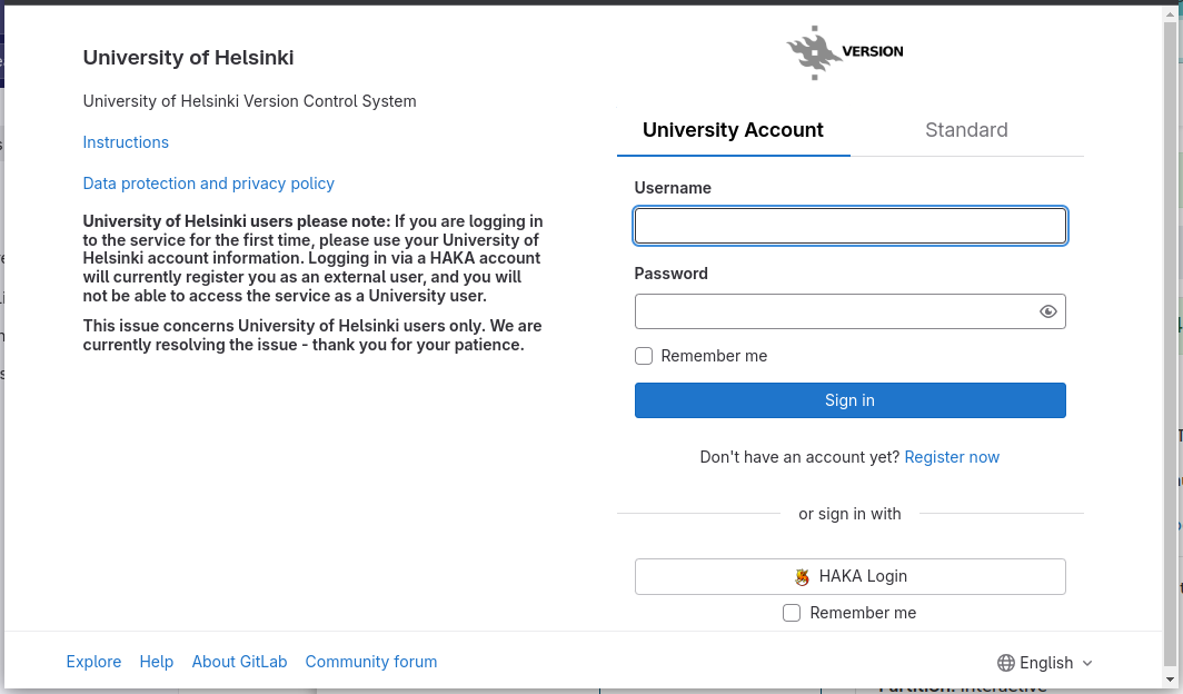
One can log into the https://version.helsinki.fi/ with the UH username and password:
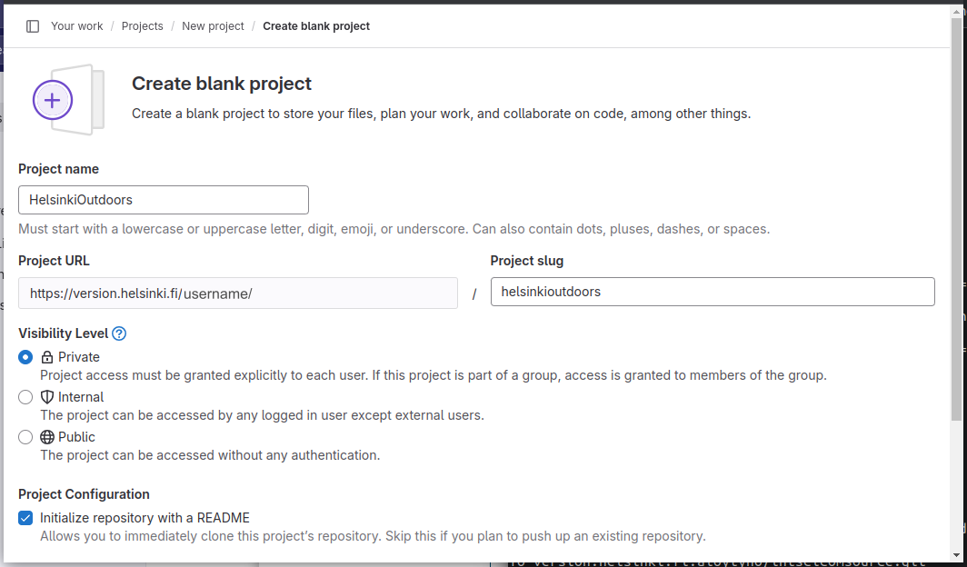
A new project is created by clicking “New project” in the top-right corner and then selecting “Create blank project”. I named this project as “HelsinkiOutdoors”, set it to be private to me and initialised the README file:
Public-private key authentication
After creating a project at GitLab (here known as the “host”), we need to be able to read the data in the host repository and write new data there from a remote computer (here known as the “client”). To prevent others reading and writing, the host has to identify the client. For this, one typically uses the SSH public-private key authentication.
The idea of the public-private key authentication is that, using the client’s public key, the host can make a question (encryption of some data) that can only be answered (decrypted to its original form) by knowing the private key; if the answer to the host’s question is correct, the person claiming to be the client must be the correct client. It is perfectly safe (and necessary) to show and distribute one’s public key but one should never share the private key. If that is shared, others can also answer correctly to the host’s question and pretend to be the intended client.
  flowchart RL
    S o-.-> |1. encrypted question|C
    S(Host<br/>public key<br/> --  ) === I((Internet)) === C(Client<br/>public key<br/>private key)
    C o-.-> | 2. decrypted answer |S
To use the public-private key authentication, we need to save a public key to the UH GitLab server; the server can then utilise this public key to generate a question that only the right person (“client”) can answer and this person is then granted access to the GitLab repository. For that, we first generate an ssh-key. This can be done with the following command and then pressing <Enter> twice to give an empty passphrase:
> ssh-keygen -f /users/$USER/.ssh/id_gitlab -t ed25519Generating public/private ed25519 key pair.
Enter passphrase (empty for no passphrase):
Enter same passphrase again:
Your identification has been saved in /users/username/.ssh/id_gitlab.
Your public key has been saved in /users/username/.ssh/id_gitlab.pub.
The key fingerprint is:
<some more lines>We can now show the public key with the command:
> cat ~/.ssh/id_gitlab.pub ssh-ed25519 AAAAC3Nza.....(Although it is perfectly safe to show the public key, I don’t show mine so that nobody accidentally copies that instead of their own key. However, one should never share the private key ~/.ssh/id_gitlab.)
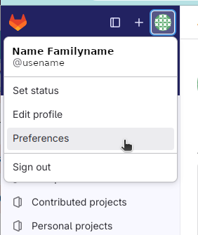
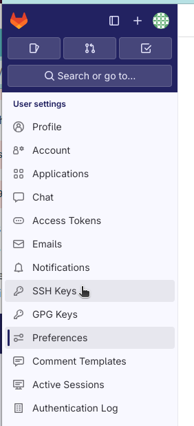
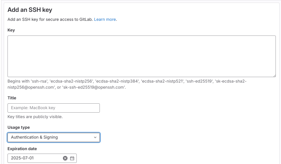
Once generated, the public key has to be copied to the host. This is done e.g. by opening “Preferences” in the left-top corner of the GitLab interface and then clicking “SSH keys”:
Invent a name (“Title”) for the key and then copy-paste the output of cat ~/.ssh/id_gitlab.pub in the “Key” box. If you wish so, set “Expiration date” futher to the future (by default one year) and click “Add key”:
Finally, we need to tell ssh to use that particular key for the GitLab server at ‘version.helsinki.fi’. We can do that by adding the information in the SSH config file:
> cat >> ~/.ssh/config << EOF
Host version.helsinki.fi
  PreferredAuthentications publickey
  IdentityFile ~/.ssh/id_gitlab
EOF
and securing this file by removing the read and write permissions from other users:
> chmod go-rw ~/.ssh/config
SSH config file
Above, the command starting with cat >> ~/.ssh/config << EOF extends an existing config file or, if such doesn’t exist, creates a new config. If something were to go wrong, repeating the above command won’t fix it as the error in the config file remains in place. One can overwrite the config file with the command (i.e. by removing one of the right-arrow characters):
> cat > ~/.ssh/config << EOF
Host version.helsinki.fi
  PreferredAuthentications publickey
  IdentityFile ~/.ssh/id_gitlab
EOF
If you have never worked with SSH before, no config file exists and overwriting is safe. One can also open the file ~/.ssh/config with a text editor and do the changes manually.
Once done, we can go back to the front page of GitLab and copy the URL of the project, selecting the “Clone with SSH” option:
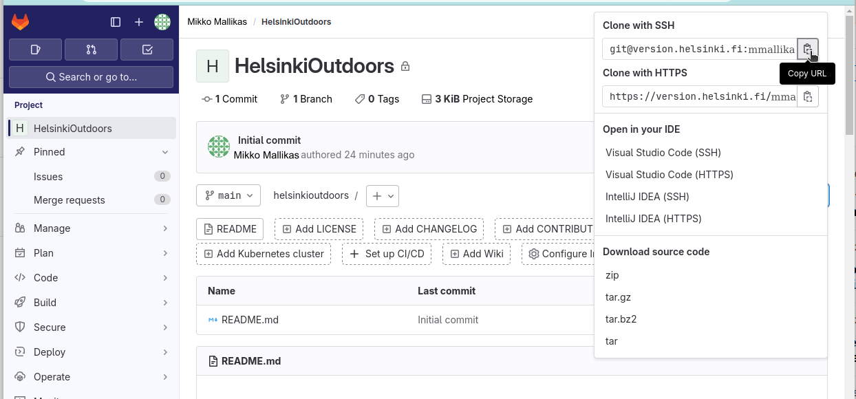
We can create the new repository under ~/IntSciCom with the following commands, pasting the URL of the repository (it should be something like git@version.helsinki.fi:username/helsinkioutdoors.git) after git clone:
> cd ~/IntSciCom/
> git clone <URL of the GitLab repository>
README file
In the project’s “homepage” at https://version.helsinki.fi/, the default view is to display the contents of the file ‘README.md’. The suffix ‘.md’ indicates that the file is written in Markdown format. It is good to read the bottom of that file, starting from “Editing this README”.
As now, the Readme file is the only content of the Git project. As we cloned the project, we also cloned this file and can read it using the command-line tools:
> cd ~/IntSciCom/helsinkioutdoors/
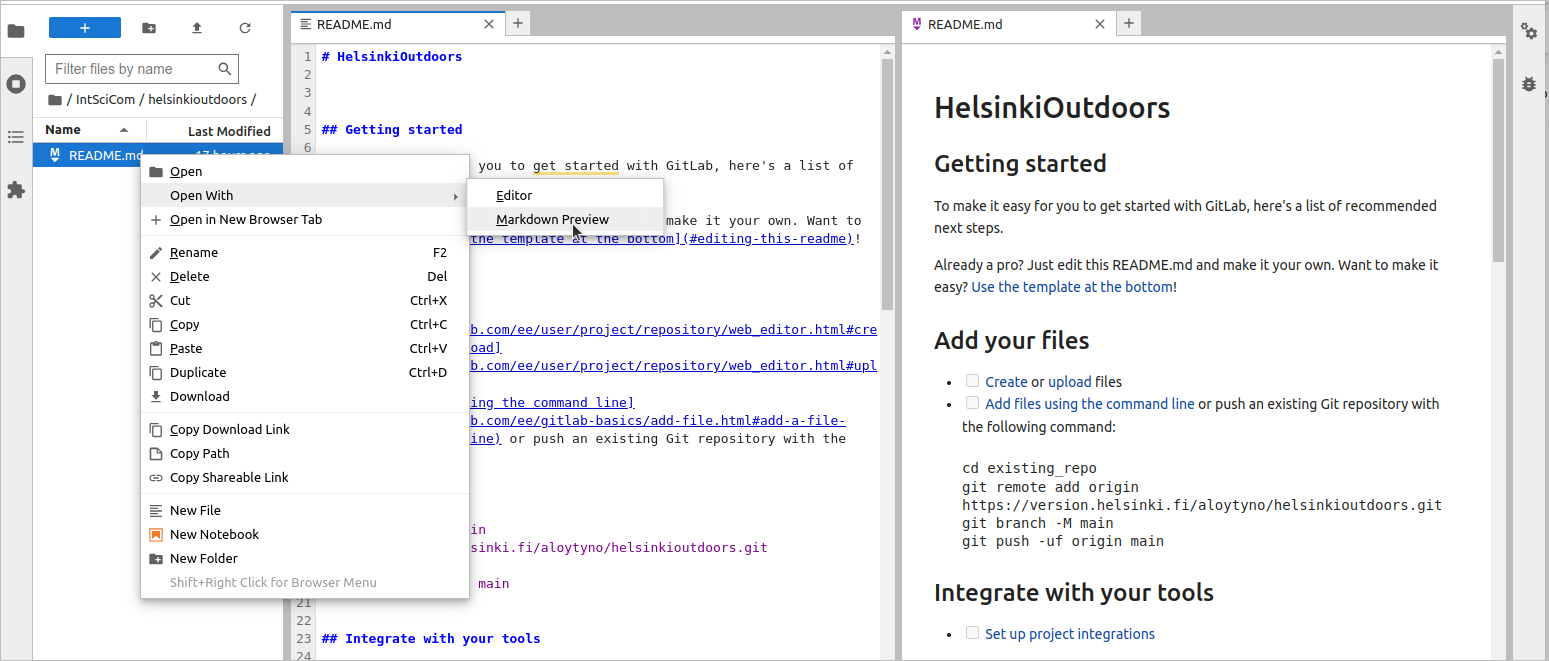
> less README.md We utilise this template for the Readme file but will edit using the Jupyter tools. For that, go to ~/IntSciCom/helsinkioutdoors/ using Jupyter’s file browser and open the file README.md (with a right-click) first with “Markdown Preview” and then with “Editor”; arrange the windows as here:
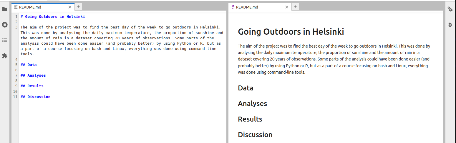
If you haven’t read the contents of the file, skim through it now. Then, delete everything until the row ## Name and, keeping in mind the instructions, start editing the remaining sections. If you don’t remember them, you can look for ideas at https://www.makeareadme.com/. Note, however, that the instructions are for software projects and, if you are doing a research project, a very different layout may be expected. Using the Jupyter text editor, I changed the content of the README.md file to be:
# Going Outdoors in Helsinki

The aim of the project was to find the best day of the week to go outdoors in Helsinki. This was done by analysing the daily maximum temperature, the proportion of sunshine and the amount of rain in a dataset covering 20 years of observations. Some parts of the analysis could have been done easier (and probably better) by using Python or R, but as a part of a course focusing on bash and Linux, everything was done using command-line tools.

## Data

## Analyses

## Results

## Discussion
I’m not sure if this will be the final layout but it’s a good starting point.
Using Git
The README.md file was in the Git project and now we changed it. We can check that git knows about it:
> git statusOn branch main
Your branch is up to date with 'origin/main'.
Changes not staged for commit:
(use "git add <file>..." to update what will be committed)
(use "git restore <file>..." to discard changes in working directory)
modified: README.md
Untracked files:
(use "git add <file>..." to include in what will be committed)
.ipynb_checkpoints/
no changes added to commit (use "git add" and/or "git commit -a")That may look gibberish but does contain information and instructions on how to proceed. To understand the message, one has to understand the basics of Git. First, we have the local files that are either “tracked” or “untracked” (top row in the diagram below); according to the message above, we have untracked files in the directory ‘.ipynb_checkpoints/’ (these are related to Jupyter and not important) while the tracked file README.md is ‘modified’ but not ‘staged’.

We can check what are the modifications with the commands:
> git diff | lessThis shows that the original text in the README.md file was replaced by the outline for the research project. We can now move these changes in the files to ‘staging area’ – that is some kind of a waiting area – with the command:
> git add README.mdNow, the status of the file has changed:
> git statusOn branch main
Your branch is up to date with 'origin/main'.
Changes to be committed:
(use "git restore --staged <file>..." to unstage)
modified: README.md
Untracked files:
(use "git add <file>..." to include in what will be committed)
.ipynb_checkpoints/Finally, we can write the changes to the repository with the command git commit; however, we need to add a description (message) telling what we have done:
> git commit -m "Updating the README.md file with the project outline"The message can be anything but it is good to make them informative as those messages are the information based on which one then searches the right point in history to recover something useful. If we do git status, we do not see anything in the tracked files but still get the message of untracked files. The contents of ‘.ipynb_checkpoints/’ will never be added to the repository and we can get rid of this useless message by telling Git that it can ignore those files. That is done by writing the file or directory name to the file .gitignore; to void Git telling about that file, we include it on the list as well:
> cat > .gitignore << EOF
.gitignore
.ipynb_checkpoints/
EOF
This repository was cloned from the UH GitLab and that remote repository is known as origin:
> git remote show origin* remote origin
Fetch URL: git@version.helsinki.fi:username/helsinkioutdoors.git
Push URL: git@version.helsinki.fi:username/helsinkioutdoors.git
HEAD branch: main
Remote branch:
main tracked
Local branch configured for 'git pull':
main merges with remote main
Local ref configured for 'git push':
main pushes to main (fast-forwardable)We can use origin as the name of the target and push our changes to the GitLab repository:
> git push originEnumerating objects: 5, done.
Counting objects: 100% (5/5), done.
Delta compression using up to 19 threads
Compressing objects: 100% (2/2), done.
Writing objects: 100% (3/3), 587 bytes | 293.00 KiB/s, done.
Total 3 (delta 0), reused 0 (delta 0), pack-reused 0
To version.helsinki.fi:username/helsinkioutdoors.git
7864083..9c3b402 main -> mainIf one now goes to the project’s page at https://version.helsinki.fi/ (and possibly refresh the view), one should see that the changes have been pushed there. By clicking the “History” button, one can study the history of the only file we currently have in the project.
Research project
In computational analyses, everything should be both human- and computer-readable. It is good to divide the data and files into categories using directories; if the project is large, these can be divided further into subdirectories. It may be beneficial to divide the documentation into multiple parts and e.g. have a Readme-file of their own in the different subdirectories. As we have seen already, it helps to use the Markdown format when writing the files. One can improve the structure and readability of the file just by using the Markdown headings and lists and indentation for the code segments.
Here, the project is simple and we create just three directories:
> cd ~/IntSciCom/helsinkioutdoors/
> mkdir data scripts analysis
Earlier, we have used the Heredoc format to write the scripts (and do also below), but in real research projects it would be impractical to write out all the scripts in the Readme files. As we use Git, it’s easy to have the ready-to-use scripts in the repository. It may be helpful to name the scripts such that the relative order of their usage becomes clear. However, it often happens that one splits existing scripts into two distinct ones or inserts an intermediate step in between, thus breaking the numbering of the scripts. One solution is to use numbers for the different stages of the project: here we could use the prefix ‘01_’ for the scripts related to data retrieval. One can try to make the scripts slightly more generic than required in the project itself, but it is also easy to modify existing scripts if one wants to apply them to a new task.
Data
The first task is to get data. Following the earlier idea of making generic tools where possible, we make a download script that takes the time period and the coordinates as arguments. If needed, it would be fairly easy to utilise the same script for another city:
> cat > scripts/01_download_openmeteo.sh << 'EOF'
#!/usr/bin/bash

sdate=$1
edate=$2
lat=$3
lon=$4

curl "https://archive-api.open-meteo.com/v1/archive?latitude=$lat&longitude=$lon&start_date=$sdate&end_date=$edate&hourly=temperature_2m&daily=temperature_2m_max,daylight_duration,sunshine_duration,rain_sum,snowfall_sum&timezone=auto"
EOF
After creating the script, we add the instructions for its usage in my README.md file:
The weather observation data for Kaisaniemi, Helsinki, were downloaded from [https://open-meteo.com/](https://open-meteo.com/) on 26 March, 2024, using the command:

     bash scripts/01_download_openmeteo.sh 2001-01-01 2020-12-31 60.175 24.9458 > data/kaisaniemi.json

The script arguments are the start and end date and the latitude and longitude. The script retrieves the observations for
- temperature_2m_max
- daylight_duration
- sunshine_duration
- rain_sum
- snowfall_sum
We have used jq for converting the JSON-formatted data to tsv-format. The command for that is messy and we wrap it into a script:
> cat > scripts/01_convert_json_tsv.sh << 'EOF'
#!/usr/bin/bash

infile=$1

jq -r '[.daily.time,.daily.temperature_2m_max,.daily.daylight_duration,.daily.sunshine_duration,.daily.rain_sum,.daily.snowfall_sum] | transpose[] | @tsv' < $infile
EOF
and then add the following text in the README.md file:
The JSON-formatted output was converted to tsv-format with the command:

    bash scripts/01_convert_json_tsv.sh data/kaisaniemi.json > data/kaisaniemi.tsv
The next piece of code we haven’t seen before. It uses the bash command date to convert the date field into a different format, adding also the day of the week and the week of the year information. In addition to that, it computes the percentage of the daylight time with sunshine and sums the rain and snowfall fields. As bash only supports integer computation, the calculation has to be done with bc and the resulting floating numbers are then rounded with printf command:
> cat > scripts/01_reformat_tsv.sh << 'EOF'
#!/usr/bin/bash

infile=$1

cat $infile | while read date temp light shine rain snow; do
  date=$(date --date=$date +"%d %m %G %a %V");
  shine=$(echo $shine"/"$light"*100" | bc -l | xargs printf "%.2f")
  rain=$(echo $rain"+"$snow | bc -l | xargs printf "%.2f")
  echo $date $temp $shine $rain;
done | tr ' ' '\t'
EOF
Note that the script is slower than the most others we have created so far as it needs to execute the commands date and bc (twice) for each of the 7305 rows in the data. Nevertheless, it should finish in less than a minute.
We also add the following text in the README.md file:
In the original data, the date field is in ISO format as in `2001-01-01`. This was broken into parts and the day of the week and the week of the year were added; in addition to that, the variation in the daylight length was incorporated by computing the percentage of the daylight hours with sunshine, and the separate fields for the rain and snowfall fields were summed. This format conversion was done with the command:

    bash scripts/01_reformat_tsv.sh data/kaisaniemi.tsv > data/kaisaniemi_formatted.tsv

Note that the script outputs "ISO week number" and "year of ISO week number" which may differ from the original date. See `man date` for details.
Full ‘Data’ section in the README.md file
Data
The weather observation data for Kaisaniemi, Helsinki, were downloaded from https://open-meteo.com/ on 26 March, 2024, using the command:
bash scripts/01_download_openmeteo.sh 2001-01-01 2020-12-31 60.175 24.9458 > data/kaisaniemi.jsonThe script arguments are the start and end date and the latitude and longitude. The script retrieves the observations for
- temperature_2m_max
- daylight_duration
- sunshine_duration
- rain_sum
- snowfall_sum
The JSON-formatted output was converted to tsv-format with the command:
bash scripts/01_convert_json_tsv.sh data/kaisaniemi.json > data/kaisaniemi.tsv In the original data, the date field is in ISO format as in 2001-01-01. This was broken into parts and the day of the week and the week of the year were added; in addition to that, the variation in the daylight length was incorporated by computing the percentage of the daylight hours with sunshine, and the separate fields for the rain and snowfall fields were summed. This format conversion was done with the command:
bash scripts/01_reformat_tsv.sh data/kaisaniemi.tsv > data/kaisaniemi_formatted.tsvNote that the script outputs “ISO week number” and “year of ISO week number” which may differ from the original date. See man date for details.
Analysis
The last step of the data processing was the reformatting of the table columns. To understand this, one can look inside the input and output file:
> head -2 data/kaisaniemi.tsv2001-01-01 0.7 21623.85 0.00 0.40 1.61
2001-01-02 -1.1 21747.98 0.00 0.00 0.00> head -2 data/kaisaniemi_formatted.tsv 01 01 2001 Mon 01 0.7 0.00 2.01
02 01 2001 Tue 01 -1.1 0.00 0.00In the output file, the columns are:
- day of month
- month of year
- year
- day of week
- week of year
- max. temperature
- percentage sunshine
- total rain/snow
To find the best day of the week to go outdoors, we want to maximise the temperature (in fact, I quite like cross-country skiing and this may not be ideal for that!) and the sunshine and minimise the rain. These are in columns 6, 7 and 8. We could write a separate script for each column but with some additional tricks we can do that with a single bash script and some awk-magic.
An important detail in the script below is to pass arguments to an awk program. The script itself takes three arguments were the second is called “field” (meaning the column in the table) and the third is called “sign” (which is supposed to be “min” or “max”). These arguments are then passed to awk with an argument like -v field=$field that assigns the awk variable (on the left side) the value of bash variable (on the right side). Inside awk, we have $field that convert the number (of field) into the column variable. We can create the script with the command:
> cat > scripts/02_get_optimal_weekday.sh << 'EOF'
#!/usr/bin/bash

infile=$1
field=$2
sign=$3

cat $infile | awk -v field=$field -v sign=$sign '
  {
    if(length(var[$3.$5])==0 ||
          $field>var[$3.$5] && sign=="max" ||
              $field<var[$3.$5] && sign=="min"){
      var[$3.$5]=$field
      day[$3.$5]=$4
    } else if($field==var[$3.$5]){
      day[$3.$5]=day[$3.$5]" "$4
    }
  }
  END{
    for(d in day){print day[d]}
  }' | tr ' ' '\n' | sort | uniq -c | awk '{print $2,$1}'
EOF
As instructions for the use of this script, we add the following text in the README.md file:
Given the formatted input data, the optimal day regarding the temperature, sunshine and rain were computed with the commands:

    bash scripts/02_get_optimal_weekday.sh data/kaisaniemi_formatted.tsv 6 max > analysis/max_temp.txt

    bash scripts/02_get_optimal_weekday.sh data/kaisaniemi_formatted.tsv 7 max > analysis/max_shine.txt

    bash scripts/02_get_optimal_weekday.sh data/kaisaniemi_formatted.tsv 8 min > analysis/min_rain.txt

These commands output the results into the files:

- analysis/max_temp.txt
- analysis/max_shine.txt
- analysis/min_rain.txt
Full ‘Analysis’ section in the README.md file
Analyses
Given the formatted input data, the optimal day regarding the temperature, sunshine and rain were computed with the commands:
bash scripts/02_get_optimal_weekday.sh data/kaisaniemi_formatted.tsv 6 max > analysis/max_temp.txt

bash scripts/02_get_optimal_weekday.sh data/kaisaniemi_formatted.tsv 7 max > analysis/max_shine.txt

bash scripts/02_get_optimal_weekday.sh data/kaisaniemi_formatted.tsv 8 min > analysis/min_rain.txt
These commands output the results into the files:
- analysis/max_temp.txt
- analysis/max_shine.txt
- analysis/min_rain.txt
Results
After running the analyses, one has to collect and process the results. In small, simple project, this can be done manually and, even in larger projects, doing it once may be far quicker if performed manually. However, a time-consuming step may raise the bar for re-running the analyses even when that would be needed and thus it is a good practice to make the whole analysis pipeline – including the collection and processing of the results – easy to re-run and replicate. On the other hand, every step of automation is a potential place for an error and, every now and then, it is good to compare computationally generated results to manually compiled ones.
In this analysis, we only have three simple output files. The counts (the number of times the day of the week has the maximum or minimum value for the given observation type) are ordered alphabetically by the name of the day, starting from Friday and ending at Wednesday. It would be fairly easy to combine the three tables and re-order the rows. For the sake of practice, we do it here computationally.
The script below uses two temporary files such that the first file is joined with one of the result files and a new file created; the new file then replaces the first file and the next file processed. In that loop, variables for the table header and a horizontal ruler are extended and, in the end, these all are combined and printed in a format suitable for a Markdown document. It would be trivial to convert the output to csv or tsv format and import it to R or a spreadsheet program. The whole script looks like this:
> cat > scripts/03_create_table.sh << 'EOF'
#!/usr/bin/bash

cat > temp_table1.txt << FEM
Fri 5
Mon 1
Sat 6
Sun 7
Thu 4
Tue 2
Wed 3
FEM

header="Day Pos"
hrule="--- ---"
for file in "$@"; do
  join -j1 temp_table1.txt $file > temp_table2.txt
  mv temp_table2.txt temp_table1.txt
  header="${header} $(basename $file .txt) "
  hrule="${hrule} ---"
done

(echo $header && echo $hrule && ( cat temp_table1.txt | sort -k2n )) | cut -d' ' -f1,3- | column -t -o ' | '
rm temp_table[12].txt
EOF
The script can take any number of output files (though it doesn’t do any checks to ensure the correct input format) and these can be either listed or given with a wildcard expansion (the same as listing the files in alphabetical order). At the simplest, the script can be run as:
> bash scripts/03_create_table.sh analysis/*Day | max_shine | max_temp | min_rain
--- | --- | --- | ---
Mon | 174 | 222 | 456
Tue | 128 | 142 | 448
Wed | 159 | 131 | 472
Thu | 136 | 117 | 456
Fri | 146 | 140 | 470
Sat | 167 | 131 | 482
Sun | 200 | 218 | 487The table is fairly easy to read but, crucially, it can be directly pasted to a Markdown document, producing this output:
| Day | max_shine | max_temp | min_rain |
|---|---|---|---|
| Mon | 174 | 222 | 456 |
| Tue | 128 | 142 | 448 |
| Wed | 159 | 131 | 472 |
| Thu | 136 | 117 | 456 |
| Fri | 146 | 140 | 470 |
| Sat | 167 | 131 | 482 |
| Sun | 200 | 218 | 487 |
In the case your results don’t quite match…
I rerun the analyses on a later date and got slightly different results. I don’t understand the reasons for this (could be e.g. changes in the original data, different versions of software on my laptop and CSC, mistakes). Nevertheless, the results are qualitatively similar and the conclusions still hold.
Double-checking script-generated results
To be honest, I didn’t believe in the results and suspected that there must be some error, possibly caused by Sunday being the last day of the week. I replicated the analyses with R and got the same results:
library(dplyr)

dat <- read.table("data/kaisaniemi_formatted.tsv")
colnames(dat) <- c("day","month","year","wday","week","temp","shine","rain")

dat %>% group_by(year,week) %>% filter(shine== max(shine)) %>% ungroup() %>% select(wday) %>% table()
dat %>% group_by(year,week) %>% filter(temp == max(temp)) %>% ungroup() %>% select(wday) %>% table()
dat %>% group_by(year,week) %>% filter(rain == min(rain)) %>% ungroup() %>% select(wday) %>% table()
wday
Fri Mon Sat Sun Thu Tue Wed
146 174 167 200 136 128 159
wday
Fri Mon Sat Sun Thu Tue Wed
140 222 131 218 117 142 131
wday
Fri Mon Sat Sun Thu Tue Wed
470 456 482 487 456 448 472 A potential explanation could be that the weather in the spring and autumn are different and this then affects the pattern within one week (in the spring, Sunday is “closest” to the coming summer; in the autumn, Sunday is “furthest” of the past summer). I’m not sure about that and maybe there’s something obvious that I don’t see. Could the traffic pollution affect the sunshine measurements?
Nevertheless, statistically speaking Sundays are good days to go outdoors in Helsinki!
Full ‘Results’ section in the README.md file
Results
The results of the three analyses were merged using the command:
bash scripts/03_create_table.sh analysis/*.txt > analysis/combined_table.md The resulting table shows the number of times the corresponding day of the week (rows) had the maximum or minimum value for the given observation type (columns) in that week. As multiple days may share the same value (especially, “rain=0”), te total count per column can far exceed the number of days within the 20 years observation period (7305 days).
| Day | max_shine | max_temp | min_rain |
|---|---|---|---|
| Mon | 174 | 222 | 456 |
| Tue | 128 | 142 | 448 |
| Wed | 159 | 131 | 472 |
| Thu | 136 | 117 | 456 |
| Fri | 146 | 140 | 470 |
| Sat | 167 | 131 | 482 |
| Sun | 200 | 218 | 487 |
Sunday appeared to the overall winner: it has clearly the greatest amount of sunshine, the second-highest temperature after Monday and the least rain.
More version control with Git
After the analyses, my directory looks like this:
> ls *README.md
analysis:
combined_table.md max_shine.txt max_temp.txt min_rain.txt
data:
kaisaniemi_formatted.tsv kaisaniemi.json kaisaniemi.tsv
scripts:
01_convert_json_tsv.sh 01_reformat_tsv.sh 03_create_table.sh
01_download_openmeteo.sh 02_get_optimal_weekday.shWhich of these files should we include in the Git repository? Normally, the practice is not to include large data files or easily reproducible files. In fact, GitHub and GitLab do not accept large files and typically the data should be stored somewhere else – and they can be obtained computationally from there. Even locally, large files cause problems as Git has to keep a copy of all the data; this data is in the local directory .git/ and tracking large data files just creates another copy of them there.
In our analysis, everything should be reproducible and, in that sense, only the scripts are truly needed. However, only the file kaisaniemi.json is large (4.3 MiB) and all other files make together around 600 KB. That is something we could easily store in a GitHub/GitLab repository (in fact, GitHub blocks files larger than 100 MiB and we could store everything there). Furthermore, one could consider the file kaisaniemi.tsv as the original unmodified data (we only changed the format) that should be stored as the reference: if we later notice that we made an error in the reformatting step, we could replicate the analysis from the “raw” data.
We can check the situation with git status:
> git statusOn branch main
Your branch is up to date with 'origin/main'.
Changes not staged for commit:
(use "git add <file>..." to update what will be committed)
(use "git restore <file>..." to discard changes in working directory)
modified: README.md
Untracked files:
(use "git add <file>..." to include in what will be committed)
analysis/
data/
scripts/
no changes added to commit (use "git add" and/or "git commit -a")Given that, we can add the missing files – and check that they got included – with the commands:
> git add data/*tsv scripts/ analysis/
> git ls-files
README.md
analysis/combined_table.md
analysis/max_shine.txt
analysis/max_temp.txt
analysis/min_rain.txt
data/kaisaniemi.tsv
data/kaisaniemi_formatted.tsv
scripts/01_convert_json_tsv.sh
scripts/01_download_openmeteo.sh
scripts/01_reformat_tsv.sh
scripts/02_get_optimal_weekday.sh
scripts/03_create_table.shgit status shows that previously untracked files are now tracked and are moved directly to the staging area:
> git statusOn branch main
Your branch is up to date with 'origin/main'.
Changes to be committed:
(use "git restore --staged <file>..." to unstage)
new file: analysis/combined_table.md
new file: analysis/max_shine.txt
new file: analysis/max_temp.txt
new file: analysis/min_rain.txt
new file: data/kaisaniemi.tsv
new file: data/kaisaniemi_formatted.tsv
new file: scripts/01_convert_json_tsv.sh
new file: scripts/01_download_openmeteo.sh
new file: scripts/01_reformat_tsv.sh
new file: scripts/02_get_optimal_weekday.sh
new file: scripts/03_create_table.sh
Changes not staged for commit:
(use "git add <file>..." to update what will be committed)
(use "git restore <file>..." to discard changes in working directory)
modified: README.md
Untracked files:
(use "git add <file>..." to include in what will be committed)
data/kaisaniemi.jsonHowever, the output reveals that the changes in README.md are not in the staging area and would not be updated to the repository; as shown before, we should do git add README.md to include it.
However, there is a shortcut, git commit -a, to include all the changes (i.e. move them to the staging area) before doing the commit. With that, we can do:
> git commit -a -m "Adding data, scripts and analysis files; updates to READM.mdE file (Discussion still missing)" 12 files changed, 14761 insertions(+)
create mode 100644 analysis/combined_table.md
create mode 100644 analysis/max_shine.txt
create mode 100644 analysis/max_temp.txt
create mode 100644 analysis/min_rain.txt
create mode 100644 data/kaisaniemi.tsv
create mode 100644 data/kaisaniemi_formatted.tsv
create mode 100644 scripts/01_convert_json_tsv.sh
create mode 100644 scripts/01_download_openmeteo.sh
create mode 100644 scripts/01_reformat_tsv.sh
create mode 100644 scripts/02_get_optimal_weekday.sh
create mode 100644 scripts/03_create_table.shOne could now run git status to see that all changes were included. One could also include data/kaisaniemi.json in .gitgnore to get rid of the notice in the output.
Finally, we push the changes and the new files to GitLab:
> git push originEnumerating objects: 19, done.
Counting objects: 100% (19/19), done.
Delta compression using up to 40 threads
Compressing objects: 100% (17/17), done.
Writing objects: 100% (17/17), 175.73 KiB | 3.38 MiB/s, done.
Total 17 (delta 0), reused 0 (delta 0), pack-reused 0
To version.helsinki.fi:username/helsinkioutdoors.git
9c3b402..2390599 main -> mainOne can then go to https://version.helsinki.fi/ and check that everything truly got there.
Version histories git Git
Our project above was a very simple exercise that tried to combine two things, the structure of a data analysis project and the usage of Git, into one case. In reality, it would made have sense to regularly update the Git repository after each major progress step. On the other hand, the commits should represent something useful and, if creating a software, it typically doesn’t make sense to commit something that is badly broken or unfinished.
Diff and log
To have a quick look at studying the file version history with Git, we wrap up our project:
> echo "Let's go for a walk on this Sunday!" >> README.md
> git commit -a -m "Finalising the project"
After this, the command git status would not show any uncommitted changes in the local files (test that!), but git log would reveal that the local and remote repositories are not in sync:
> git log --onelined15f7fb (HEAD -> main) Finalising the project
2390599 (origin/main, origin/HEAD) Adding data, scripts and analysis files; updates to READM.mdE file (Discussion still missing)
9c3b402 Updating the README.md file with the project outline
7864083 Initial commitIn the output, the first word is the hash code of the node in the history and after that comes the commit message. In between these two, the words in brackets tell the status of the different repositories: “HEAD” is the pointer to the current location in the local history and “main” is the default branch (see below a bit more about this). Those starting with “origin/” are the same for the remote repository (please recall the command git remote show origin from above). We can get the two in sync by pushing the local changes to GitLab:
> git push originEnumerating objects: 5, done.
Counting objects: 100% (5/5), done.
Delta compression using up to 19 threads
Compressing objects: 100% (3/3), done.
Writing objects: 100% (3/3), 415 bytes | 207.00 KiB/s, done.
Total 3 (delta 1), reused 0 (delta 0), pack-reused 0
To version.helsinki.fi:username/helsinkioutdoors.git
2390599..d15f7fb main -> mainand then:
> git log --onelined15f7fb (HEAD -> main, origin/main, origin/HEAD) Finalising the project
2390599 Adding data, scripts and analysis files; updates to READM.mdE file (Discussion still missing)
9c3b402 Updating the README.md file with the project outline
7864083 Initial commitWe can see the difference between two time points in the history with the command git diff <hash1> <hash2> <filename>. Here, we study the difference between the second last and the last commit in the file “README.md”:
> git diff d15f7fb 2390599 README.md diff --git a/README.md b/README.md
index 4a622c0..b831ed4 100644
--- a/README.md
+++ b/README.md
@@ -64,3 +64,4 @@ Sun | 200 | 218 | 487
Sunday appeared to the overall winner: it has clearly the greatest amount of sunshine, the second-highest temperature after Monday and the least rain.
## Discussion
+Let's go for a walk on this Sunday!The output is familiar from the program diff that was used earlier. Note that “HEAD” is a valid name for a time point and we could have equally well written git diff d15f7fb HEAD README.md
Commands with hash names
The hash names (such as “d15f7fb” and “2390599” above) are unique to each project and one should adjust all the commands to match the true hash names in the local project.
Going truly back to history
After finishing the project, the local files look like this:
> ls *README.md
analysis:
combined_table.md max_shine.txt max_temp.txt min_rain.txt
data:
kaisaniemi_formatted.tsv kaisaniemi.json kaisaniemi.tsv
scripts:
01_convert_json_tsv.sh 01_download_openmeteo.sh 01_reformat_tsv.sh 02_get_optimal_weekday.sh 03_create_table.shEarlier, we outputted the log of commits:
> git log --onelined15f7fb (HEAD -> main) Finalising the project
2390599 (origin/main, origin/HEAD) Adding data, scripts and analysis files; updates to READM.mdE file (Discussion still missing)
9c3b402 Updating the README.md file with the project outline
7864083 Initial commitUsing the commit hash names, we can go back to any stage in the commit history with the command git checkout. Here, we go back to “9c3b402” where the commit message is “Updating the README.md file with the project outline”:
> git checkout 9c3b402Note: switching to '9c3b402'.
You are in 'detached HEAD' state. You can look around, make experimental
changes and commit them, and you can discard any commits you make in this
state without impacting any branches by switching back to a branch.
If you want to create a new branch to retain commits you create, you may
do so (now or later) by using -c with the switch command. Example:
git switch -c <new-branch-name>
Or undo this operation with:
git switch -
Turn off this advice by setting config variable advice.detachedHead to false
HEAD is now at 9c3b402 Updating the README.md file with the project outlineIndeed, the file “README.md” only contains the project outline:
> cat README.md # Going Outdoors in Helsinki
The aim of the project was to find the best day of the week to go outdoors in Helsinki. This was done by analysing the daily maximum temperature, the proportion of sunshine and the amount of rain in a dataset covering 20 years of observations. Some parts of the analysis could have been done easier (and probably better) by using Python or R, but as a part of a course focusing on bash and Linux, everything was done using command-line tools.
## Data
## Analyses
## Results
## DiscussionWe can use ls to check that this is indeed the start of the project where all the scripts and data files were missing:
> ls *README.md
data:
kaisaniemi.jsonNote that the file “kaisaniemi.json” is in place as it not tracked by Git and thus not affected by the git commands.
We can get back to the current status of the project with git checkout main:
> git checkout mainPrevious HEAD position was 9c3b402 Updating the README.md file with the project outline
Switched to branch 'main'
Your branch is up to date with 'origin/main'.Now, all the files created during the research project are again in place
> ls *README.md
analysis:
combined_table.md max_shine.txt max_temp.txt min_rain.txt
data:
kaisaniemi_formatted.tsv kaisaniemi.json kaisaniemi.tsv
scripts:
01_convert_json_tsv.sh 01_download_openmeteo.sh 01_reformat_tsv.sh 02_get_optimal_weekday.sh 03_create_table.sh> tail README.md Wed | 159 | 131 | 472
Thu | 136 | 117 | 456
Fri | 146 | 140 | 470
Sat | 167 | 131 | 482
Sun | 200 | 218 | 487
Sunday appeared to the overall winner: it has clearly the greatest amount of sunshine, the second-highest temperature after Monday and the least rain.
## Discussion
Let's go for a walk on this Sunday!We can also restore the historical version of a specific file. Here, we go back to an earlier version of README.md and then back to the latest one; we use the word count (wc) to see the changes in the:
> wc README.md 67 498 3402 README.md> git checkout 9c3b402 README.mdUpdated 1 path from e1c00bd> wc README.md 10 94 522 README.md> git checkout main README.mdUpdated 1 path from 1c6ab16> wc README.md 67 498 3402 README.mdGraphical tools
The Git history is much easier to study and understand using graphical programs. Many software development programs have integrated tools for studying the changes and many stand-alone programs exist for Windows, MacOS and Linux. The Git package contains the program gitk that is available for all platforms (though not on the CSC system). A brief introduction to gitk is available e.g. at https://devtut.github.io/git/git-gui-clients.html#gitk-and-git-gui.
Next steps with Git
Above, we used Git mainly as a backup system with the edit history – it can be very useful as such – and the exercises utilised the very rudimentary features of Git and GitLab. Below are some pointers to more advanced features.
Collaboration and merging
Typically, Git is used for collaborative work and the members should get access to the central repository. One option in GitLab is to go to “Manage” and “Members” (in the left sidebar) and invite colleagues as members in the project with a specified role (Guest, Reporter, Developer, Maintainer, Owner); they will then see the project in their own GitLab page and can set up the access as explained above,
When collaborating, the members of the project can edit the files and push the changes in the repository; once there, others can then pull the changes to their local repository and files. If the parallel changes are affecting different parts of the files, Git typically can combine them into a consensus. This is known as “merging”. For the merging to work optimally, it is crucial to push frequently and pull frequently. Sometimes the parallel edits clash and someone has to merge the files manually. In practice, Git provides the two alternatives (e.g. two alternative versions of a sentence) in a text editor and one then has to combine these into an acceptable compromise (it can of course be one of the alternatives), save the file and commit it. It’s not too scary and can be learned by doing.
Testing with branches
Our Git history was incremental and linear. It is very common to make sidetracks, known as “branches”, and then potentially merge these branches with the main branch. A branch can be an experiment that potentially fails and the benefit of isolating that experiment into a branch is the ease of abandoning the work and returning to starting point. When writing a text, one may wonder whether swapping the order of two paragraphs would clarify the flow of reasoning. It would be easy to create a branch for that, make the changes and then decide if it is better or worse than the original one. Jumping between different branches is done using git checkout and it doesn’t technically much differ from jumps in the history between commit points.
Local Git repositories
Above, we created the project in GitLab and then cloned that to a local repository. The advantage of this is that the remote address, “origin”, is then automatically defined and pushing the changes to the server is easy. If there are no plans to store the data anywhere else, it is better to create the repository locally. That is done with git init:
> cd ~/IntSciCom
> mkdir AnotherProject
> cd AnotherProject
> git init
hint: Using 'master' as the name for the initial branch. This default branch name
hint: is subject to change. To configure the initial branch name to use in all
hint: of your new repositories, which will suppress this warning, call:
hint:
hint:   git config --global init.defaultBranch <name>
hint:
hint: Names commonly chosen instead of 'master' are 'main', 'trunk' and
hint: 'development'. The just-created branch can be renamed via this command:
hint:
hint:   git branch -m <name>
Initialized empty Git repository in /users/username/IntSciCom/AnotherProject/.git/
The message above indicates that this is an old version Git and the default branch is still called “master”. In computing, many systems have one “boss” (that controls the overall flow of things) and potentially many “underlings” (that follow the commands) and these have been traditionally known as “master” and “slave(s)”. Recently, these technical terms have been increasingly criticised and, as a result, also Git changed it terminology: instead of “master”, the default branch created for a project is nowadays called “main” (it never used the term “slave”). The message above gives instructions for changing the name.
Even if not planning to share the repository, it is good to set the username and email address. This is done with git config, globally (for all projects) with the argument --global:
> git config --global user.name "Mona Lisa"
> git config --global user.email "mona.lisa@helsinki.fi"
We can then add files to be tracked and make commits like above:
> touch README.md
> git add README.md
> git commit -m "Starting a new project"
[master (root-commit) 4068c03] Starting a new project
1 file changed, 0 insertions(+), 0 deletions(-)
create mode 100644 README.md> git log --oneline4068c03 (HEAD -> master) Starting a new projectNote though that the Git-generated files (inside .git/) have write permission such that they can’t be deleted with the simple rm command; instead, the --force argument has to be used and we can delete the project and its Git repository with the commands:
> cd ~/IntSciCom
> rm -rf AnotherProject
Take-home message
Git is a central tool for everyone working on programming code and computer-based data analysis. However, Git works for any kind of text- and line-based files, for example, manuscripts written with Markdown or LaTeX. Git can also be useful when working on multiple computers and allows keeping files up-to-date.
The idea of Markdown is that the files can be easily written and read in the “raw” format but then, with software such as Pandoc, be translated into various more visual formats. Pandoc can translate Markdown to tens of other formats, including Microsoft Word and PowerPoint.
This web course was written in Markdown using Quarto (which uses Pandoc) and Visual Studio Code. VSC has plugins that facilitate compiling Markdown into a website (such as this course) or a Pdf document (manuscripts and other text documents). The resulting html-documents were managed and copied to the server computer using Git.